Projects, Leah Kat Insights

Project 5 · Hospitality

Hotel RevPAR Performance Readout

An STR-style monthly performance readout for an urban hotel: occupancy, ADR, RevPAR, and market share indices against a competitive set, built from 119,000 real bookings through a bronze/silver/gold Delta pipeline on Databricks.

Why this oneReading an STR report is a named skill in hotel revenue analyst postings, so this project uses that vocabulary throughout: RevPAR index, MPI, ARI, comp set, pace, pickup. Real booking data runs through a Databricks lakehouse built the way a production one would be, and the output is the report a GM receives each month, plus a one-page memo on what to do about it. The comp set is simulated from the source data and labeled as such on every exhibit.

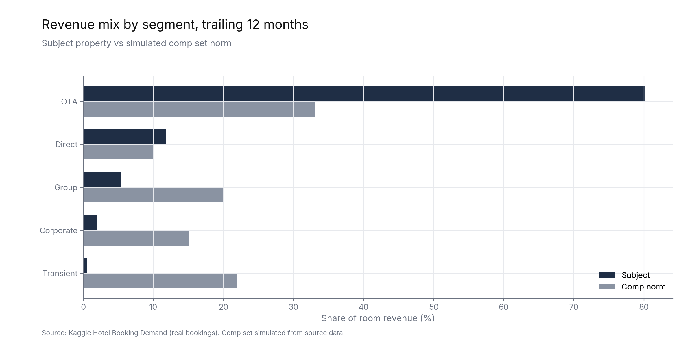
STAR-style summary table: monthly occupancy, ADR, and RevPAR for the subject property and comp set, with MPI, ARI, and RGI index rows. — The readout: subject vs comp set, six months

To the General Manager

Recommendation: hold rate. We are out-earning the comp set on RevPAR because our rate premium more than covers an occupancy gap, and the gap is specific: midweek, short-lead, corporate-adjacent business that the discounter across the street is buying. Close it with targeted corporate rate fences and a two-week booking window offer rather than blanket discounting. Cutting rate to chase MPI would give up rate we already earn to buy occupancy we can win more cheaply.

Read the one-page memo

103.5

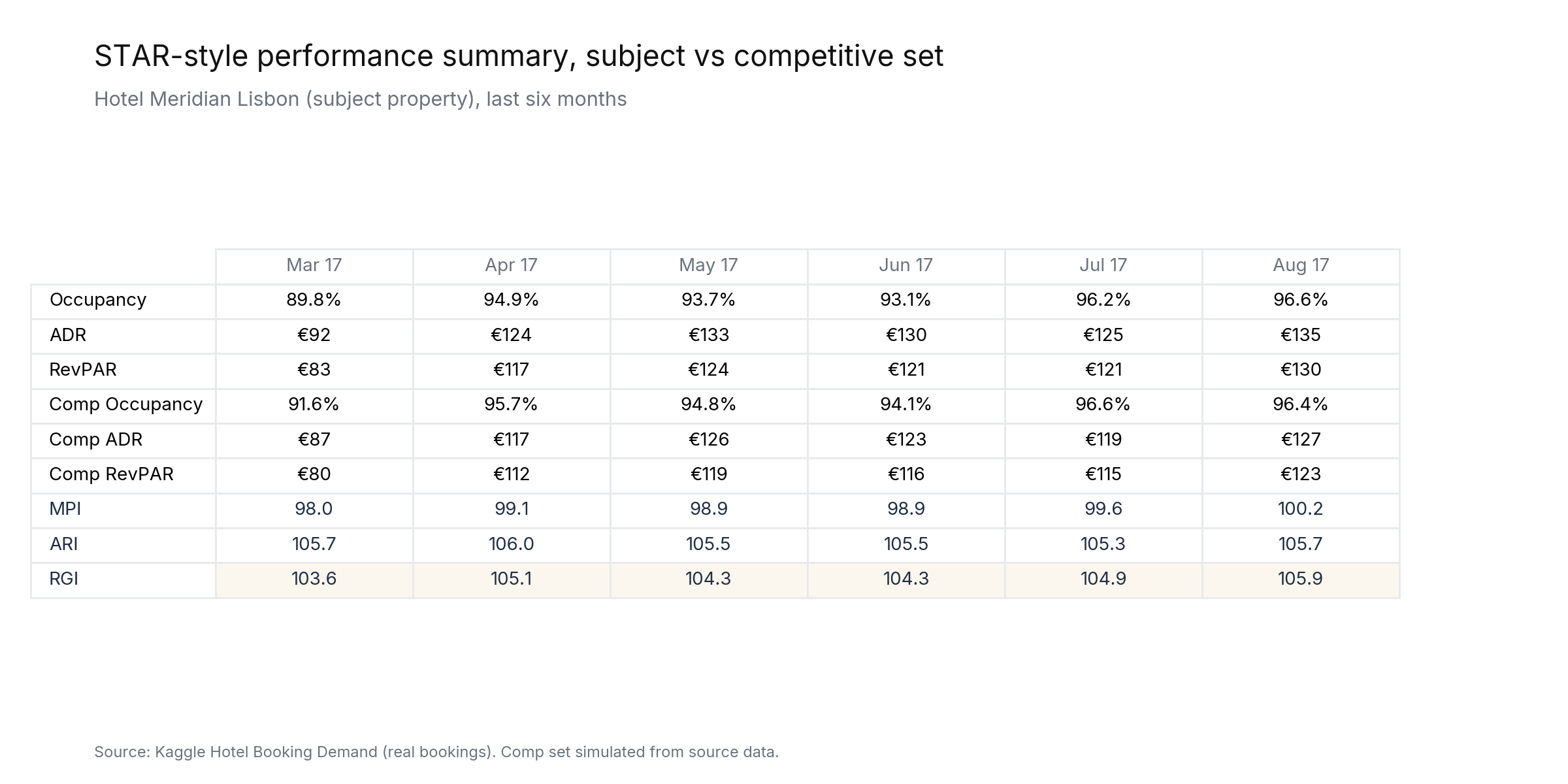
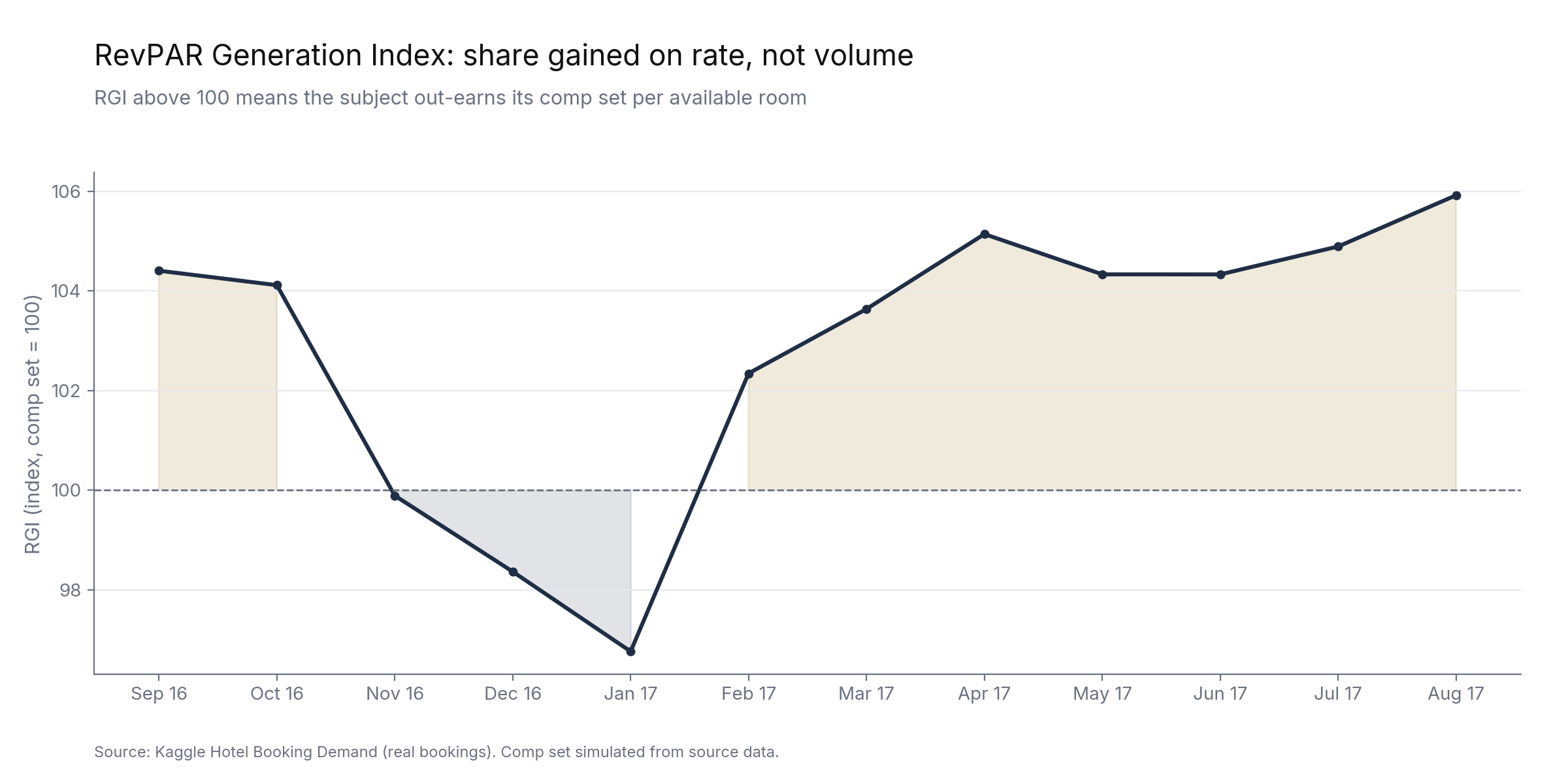
RevPAR Generation Index, trailing twelve months. Above 100 means the property earns more per available room than its comp set, so it is gaining share rather than riding the market.

106.1

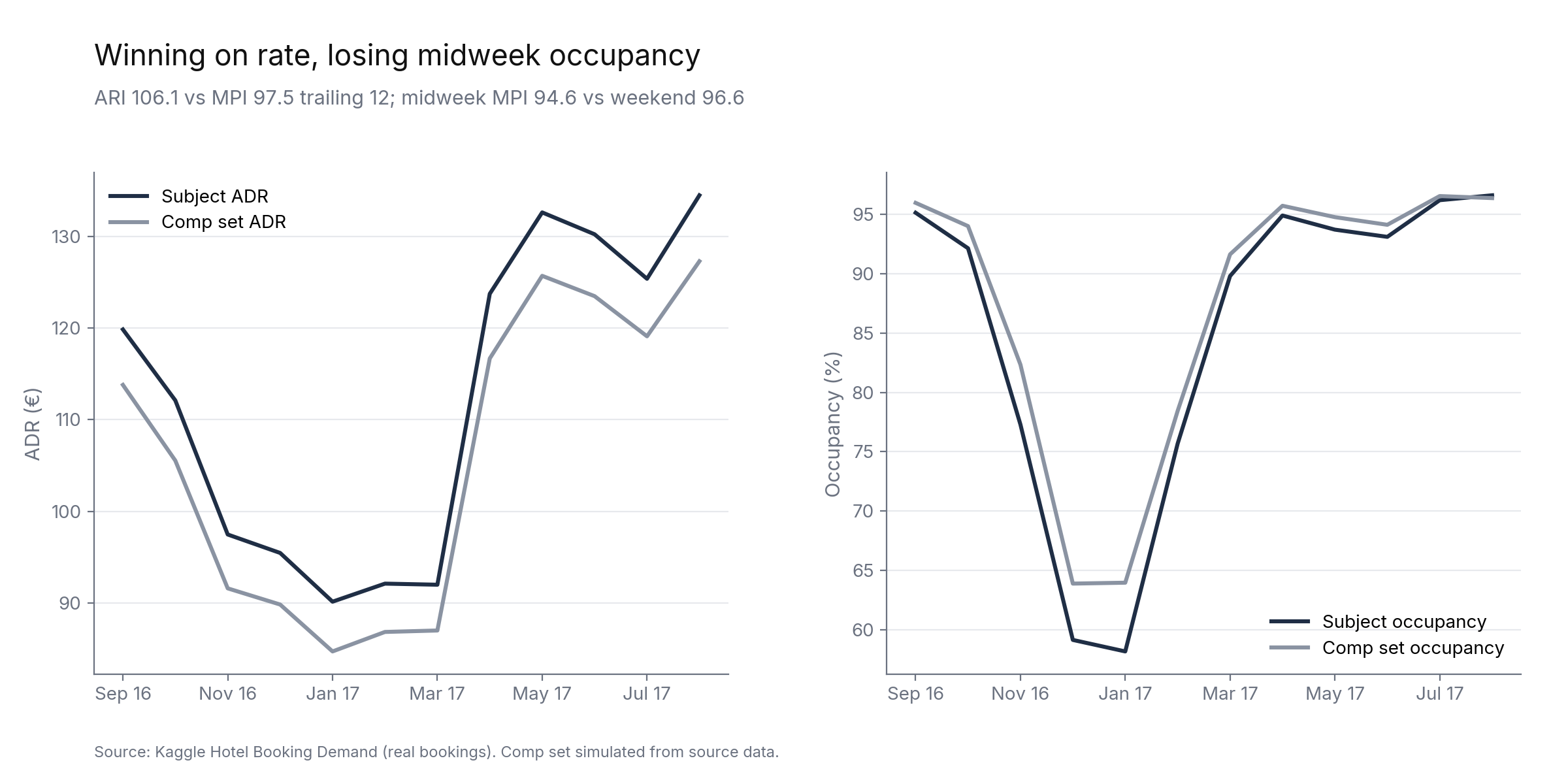
ADR index. The share gain is coming entirely from rate. The property prices above the comp set and the market keeps paying it.

97.5

Occupancy index, and the warning in the readout. The rate premium costs heads in beds, and the gap concentrates midweek, where the discounter comp is buying occupancy.

RGI trend over twelve months with the 100 index line marked and share gain shaded. — RGI: share gain over 12 months

Side-by-side ADR and occupancy trends for subject property versus comp set. — The decomposition: rate vs occupancy

Revenue mix by market segment, subject property versus simulated comp set norm. — Segment mix vs comp norm

Booking pace curves: share of final room nights on the books by days before arrival, 2017 versus 2016. — Pace: real lead-time data, 2017 vs 2016

1. CSV → Bronze Delta

119K raw bookings land in a Unity Catalog volume and are written to a bronze Delta table untouched, with an ingestion timestamp added. Bronze is just the landing zone.

2. Silver: one row, one booking

Arrival dates assembled from parts, cancellations typed, zero-guest and negative-rate rows dropped, the famous €5,400 ADR outlier capped, market segments normalized to five clean values. Data-quality checks stop the run if any of those rules fail.

3. A simulated comp set

A readout needs a market to compare against, and the source data has none. Four competitor hotels are simulated from the subject's own daily history: one prices above the market, one discounts to fill rooms, one runs on group business, one tracks the average. Their results roll up room-weighted, the same way STR builds a comp set.

4. Gold KPIs → readout

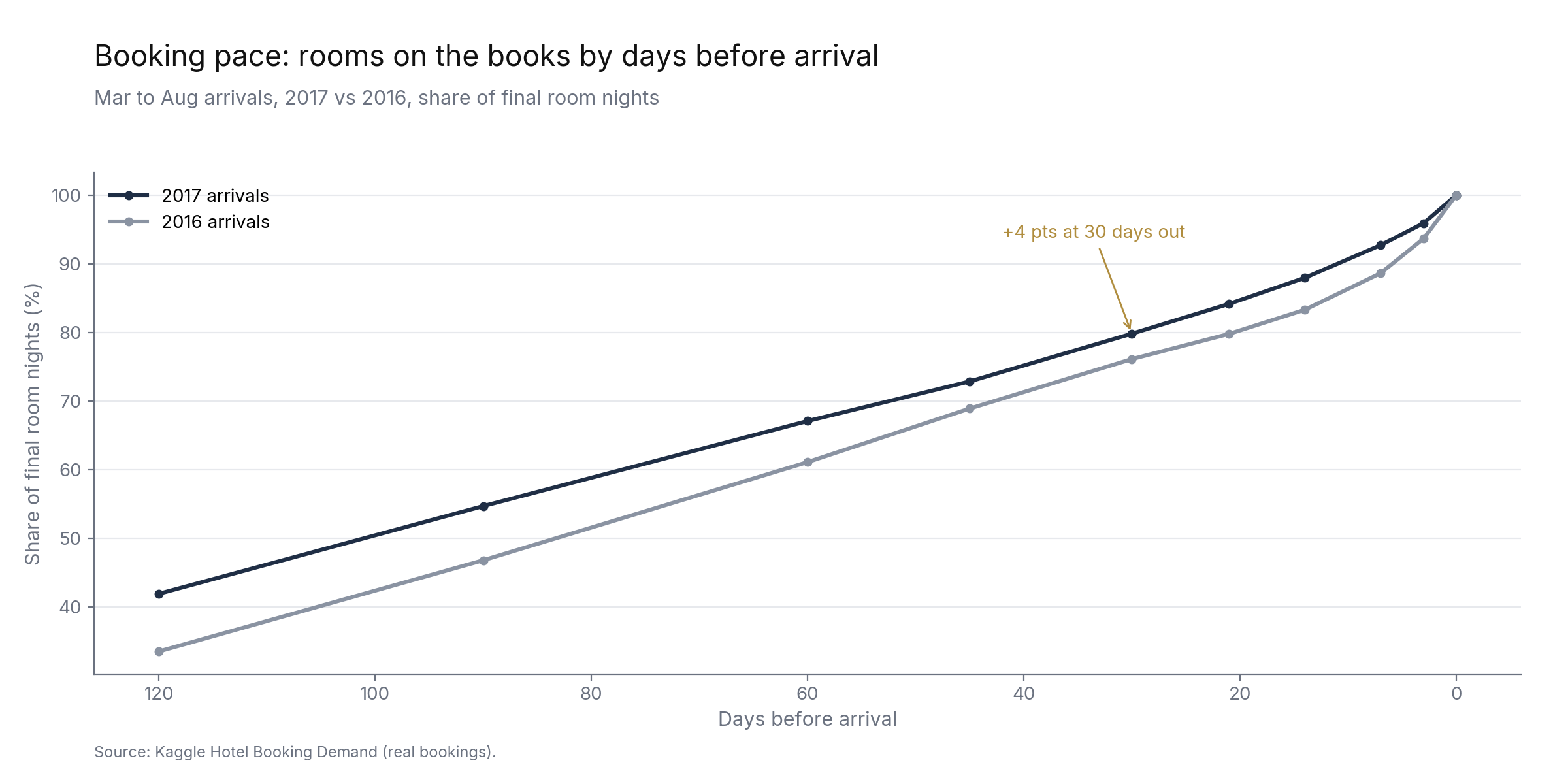
Stay-night explosion turns bookings into daily occupancy, ADR, and RevPAR. Monthly rollups add MPI, ARI, and RGI. Booking pace comes from real lead times: rooms on the books at 120, 60, 30 days out.

Pythonpandas · numpy · matplotlib

DatabricksUnity Catalog, serverless compute

Δ

Delta Lakebronze / silver / gold medallion

PySparkstay-night explosion, pace checkpoints

STR

STR conventionsMPI · ARI · RGI · comp set

pytest19 tests over every transform

Project 1

Stock Market Analytics Pipeline

End-to-end cloud data pipeline pulling live stock data, processing it through AI, and visualizing trends in a Delta Lake data lakehouse.

Stock analytics is the classic first portfolio project. This one runs on real cloud infrastructure end to end, uses an LLM (Claude via AWS Bedrock) for the analysis layer, and stores the data in a lakehouse with ACID transactions instead of a local CSV.

Monthly stock price trends from the Databricks Delta Lake table. — Databricks SQL trend output

1. Data Ingestion

Python pulls 6 months of daily price data for AAPL, TSLA, AMZN, GOOGL, MSFT via Yahoo Finance API. Cleaned, normalized, uploaded to S3 as structured CSV.

2. Serverless AI Analysis

Lambda triggers on new S3 data. Reads CSV, sends to Claude via AWS Bedrock for pattern analysis, writes AI-generated insights back to S3.

3. Delta Lake Storage

Data loaded into Databricks and saved as a Delta Lake table with ACID transactions, schema enforcement, and time travel, so any earlier version can be restored.

4. SQL Analytics & Viz

Databricks SQL surfaces monthly trends, price ranges, best and worst trading days, year-over-year comparisons. Rendered as interactive dashboards.

Pythonboto3 · pandas · yfinance

S3

AWS S3cloud object storage

λ

AWS Lambdaserverless compute

AWS BedrockClaude AI integration

Databrickslakehouse analytics

Δ

Delta Lakeversioned data storage

Project 2

Customer Lifetime Value Model

Probabilistic CLV predictions for a synthetic golf ecommerce retailer. Turned 65,000 transactions into per-customer 12-month revenue forecasts using RFM features and BG/NBD + Gamma-Gamma models.

Predicted customer lifetime value by segment: average CLV per customer on the left, total CLV per segment on the right. — CLV by segment

10.2x

Tour Enthusiasts outspend Weekend Golfers by 10.2x in predicted lifetime value, and the top two segments drive 70% of forecasted revenue from just 32% of the customer base. They cost about the same to acquire.

$3.1M

Predicted next-12-month revenue, calculated one customer at a time. Drives acquisition budget and retention priorities.

Top 10 predicted CLV customers, historical spend vs predicted next 12 months. — Top 10 predicted CLV customers

1. Synthetic Data Generation

Built a realistic golf ecommerce dataset in Python. 65,000 transactions across 5,000 customers and six behavioral segments, with seasonality, churn patterns, and upgrade cycles baked in.

2. Delta Lake Bronze Layer

Raw transactions uploaded to S3 and loaded into Databricks as a Delta table with schema enforcement, time travel, and ACID transactions.

3. RFM Feature Engineering

SQL aggregations turn raw orders into per-customer Recency, Frequency, and Monetary features. Silver layer table, one row per customer, ready for modeling.

4. BG/NBD + Gamma-Gamma

Industry-standard probabilistic CLV models. BG/NBD predicts future transaction counts. Gamma-Gamma predicts order value. Combined, they output expected 12-month revenue per customer.

Pythonpandas · numpy · lifetimes

S3

AWS S3raw data storage

DatabricksSQL · notebooks · Spark

Δ

Delta Lakemedallion architecture

βγ

BG/NBDpurchase frequency model

Γ²

Gamma-Gammamonetary value model

Project 3

Lululemon DCF Valuation Pipeline

A personal 5-year DCF valuation of Lululemon Athletica (NASDAQ: LULU), pulled from live SEC EDGAR filings and current market data. Built as a real data engineering pipeline through medallion architecture, SQL window functions, and a reverse DCF that backs out what the market is pricing in.

Why this oneThe valuation itself could be done in Excel in an afternoon. The point of the project is the pipeline: Lambda-shaped Python pulling raw XBRL from SEC, normalized through bronze/silver/gold layers, queried with SQL window functions in DuckDB (portable to a Databricks SQL warehouse), then valued with a base case plus bear/bull sensitivity. Live yfinance data anchors the reverse DCF to the current market price.

Lululemon revenue: post-COVID era history with five-year base-case projection. — Post-COVID revenue + 5-yr base case

1. SEC EDGAR → Bronze

Python pulls every XBRL fact Lululemon has ever reported from SEC EDGAR in a single API call. Filtered to the 25 line items the model needs, landed in S3 Bronze. Lambda-ready for scheduled refreshes.

2. XBRL → Silver Parquet

Pandas parser normalizes XBRL tag variants into clean column names. Handles old vs. new accounting standards, so the same parser works for Nike, Adidas, and Under Armour without edits. Output: 16 years of typed financial data as Parquet.

3. SQL Window Functions → Gold

DuckDB runs SQL window functions over the silver table to compute YoY growth, 5-year rolling CAGR, margin compression vs peak, and FCF conversion. Same SQL ports to a Databricks SQL warehouse with a one-line connection swap.

4. DCF + Reverse DCF

5-year free cash flow projection, discounted at the cost of equity, with a Gordon-growth terminal value. Reverse DCF backs out the growth, margin, and discount rate that the current market price implies.

5. Bear / Base / Bull

Three sets of growth and margin assumptions run through the same model. The output is a side-by-side valuation with every assumption listed.

18.0%

Discount rate implied by the current $117.32 market price, against an 11.9% cost of equity from CAPM. A gap that size is a distressed-company risk premium.

-9.2%

Implied revenue growth at the current price. The market is pricing in five years of revenue decline, alongside margin compression and a distressed-company discount rate.

$0

Long-term debt on the balance sheet. Lululemon runs net cash, so the model simplifies to equity-only valuation with operating leases as the only meaningful obligation.

Reverse DCF: implied revenue CAGR, operating margin, and WACC vs historical actuals. — What the market is pricing in

LULU 5-year FCFF projection under three scenarios. — FCFF: bear, base, bull

Pythonpandas · numpy · scipy · matplotlib

SEC

SEC EDGARXBRL companyfacts API

λ

AWS Lambda + S3scheduled ingest, medallion layers

DuckDBSQL window functions, Databricks-portable

scipy.optimizebrentq root finding for reverse DCF

Y!

yfinancelive price & diluted shares

Project 4 · Quick build

Multi-Channel Reorder Forecasting System

A small forecasting and decision tool for a multi-channel DTC wellness brand. A KPI overview covers revenue, units, and top movers, and a five-state reorder engine turns the sales history into a daily action list.

The math behind reorder timing usually lives in a spreadsheet, and the spreadsheet breaks as soon as a SKU goes seasonal or a second sales channel shows up. This tool replaces it. A recency-weighted velocity model handles trend and noise. A five-state machine (reorder_now / soon / healthy / slow / dead, plus an on_order override) means every decision can be traced back to its inputs. The KPI overview at the top (revenue, units, average daily sales, SKUs in scope, reorder count) gives the operator the context around each recommendation. Underneath, two sales channels are reconciled into a single per-SKU view, with vendor lead times and outstanding POs joined in. It's a Streamlit application rather than a notebook.

Overview dashboard showing KPI tiles for revenue, units sold, average daily revenue, SKUs in scope, and reorder count, with a sales trend line and category breakdown. — Overview, the operating context

Every recommendation can be opened to its inputs. The Forecast Detail view shows the velocity model, the rolling window, the days-of-supply calculation, and the recommended quantity formula side by side, so an operator who questions a number gets the answer in one click. Velocity spread between top- and bottom-quartile SKUs runs 9.0x, and recency weighting keeps fast movers reordering ahead of slow ones even when on-hand counts match.

Forecast Detail page showing per-SKU sales history, forecast projection, KPI tiles, and the math breakdown of velocity and recommended quantity. — Forecast Detail, with the math breakdown expanded

56 / 200

SKUs flagged reorder_now this cycle. Operators work a short prioritized queue each morning instead of checking all 200 SKUs by hand.

$1.18M

Recommended purchase-order value for reorder_now SKUs this cycle, grouped by vendor with MOQ already applied. Operators copy the per-vendor list straight into the PO email.

Reorder Alerts page showing per-SKU status dots, days of supply, recommended quantity, and PO value, filtered to reorder_now and reorder_soon rows. — Reorder Alerts, the morning action queue

1. Multi-Channel Sales Sync

Python pulls daily orders from Shopify Admin API and Square API, normalizes both into a single (sku, date, units, revenue) schema with a source column, and stores 365 days of rolling history.

2. Normalized Postgres Schema

Products, vendors, settings, purchase log, and forecast log live in a normalized schema with foreign keys and indexes. Schema enforces that every SKU has a vendor, lead time, MOQ, and unit cost, so the downstream math always has what it needs.

3. Weighted Rolling Velocity

90-day rolling-average sales velocity per SKU, with linear recency weighting and an optional per-SKU growth factor. Cold-start and dead SKUs are handled as explicit cases instead of coming through as zeros.

4. Five-State Reorder Engine

Days of supply is on_hand divided by velocity. Compared against target cover days plus vendor lead time to produce one of reorder_now, reorder_soon, healthy, slow, or dead. Outstanding POs override to on_order. Recommended quantity respects vendor MOQ.

5. Streamlit Operator App

Six-page application: Overview KPIs, Reorder Alerts, All Products, Forecast Detail per SKU, Purchase Log, Vendors. Filters cascade across pages. Writes a forecast_log row on every refresh for historical audit.

Pythonpandas · numpy · requests

Streamlitmulti-page operator app

PostgreSQLnormalized schema · indexes

Shopify Admin APIorders · inventory · products

Square APIorders · payments

Λ

Altairinteractive charts